CPA
Foundation Leval
Quantitative Analysis May 2016
Suggested solutions

Revision Kit

| ➧ | Quantitative Analysis -September-2015-Pilot-Paper |
| ➧ | Quantitative Analysis-November-2015-Past-Paper |
| ➧ | Quantitative Analysis-May-2016-Past-paper |
| ➧ | Quantitative Analysis-November-2016-Past-Paper |
| ➧ | Quantitative Analysis-December-2017-Past-paper |
| ➧ | Quantitative Analysis-May-2017-Past-paper |
| ➧ | Quantitative Analysis-November-2018-Past-paper |
| ➧ | Quantitative Analysis-May-2018-Past-paper |
| ➧ | Quantitative Analysis-May-2019-Past-paper |
| ➧ | Quantitative Analysis-November-2019-Past-paper |
| ➧ | Quantitative Analysis-November-2020-Past-paper |
| ➧ | Quantitative Analysis-December-2021-Past-paper |
| ➧ | Quantitative Analysis-April-2021-Past-paper |
| ➧ | Quantitative Analysis-August-2021-Past-paper |


QUESTION 1(a)
QUESTION 1(b)
QUESTION 1(c)
QUESTION 2(a)
Univariate Function: A univariate function is a mathematical function that involves only one variable. It maps each value of that variable to a unique output.
Multivariate Function: A multivariate function is a mathematical function that involves multiple variables. It maps combinations of values of these variables to unique outputs.
Univariate Function: In a univariate function, there is only one independent variable. It is represented as f(x) where x is the single variable.
Multivariate Function: In a multivariate function, there are two or more independent variables. It is represented as f(x, y, z, ) where x, y, z, are the multiple variables involved.
Univariate Function: The graph of a univariate function is typically a curve in a two-dimensional coordinate system, where one axis represents the independent variable.
Multivariate Function: The graph of a multivariate function exists in a multi-dimensional space, and visualizing it may require three or more dimensions, depending on the number of variables.
Univariate Function: f(x) = 2x + 3 where x is the independent variable.
Multivariate Function: f(x, y) = 3x^2 + 2y - 5 where x and y are the independent variables.
Univariate Function: Univariate functions are one-dimensional, involving a single variable.
Multivariate Function: Multivariate functions are multi-dimensional, involving two or more variables.
Univariate Function: Derivatives in a univariate function are calculated with respect to a single variable, yielding a rate of change with respect to that variable.
Multivariate Function: Partial derivatives in a multivariate function are calculated with respect to each variable independently, providing rates of change with respect to individual variables.
Univariate Function: Represented as f(x) or y = f(x), where x is the independent variable.
Multivariate Function: Represented as f(x, y) or z = f(x, y) , where x and y are the independent variables.
Univariate Function: Commonly used in modeling relationships involving a single variable, such as distance as a function of time.
Multivariate Function: Applied in scenarios where multiple factors influence an outcome, such as the temperature as a function of both time and geographical location.
Univariate Function: Typically expressed as an equation involving a single variable, and solutions are points on a one-dimensional axis.
Multivariate Function: Involves equations with multiple variables, and solutions are points in a multi-dimensional space.
Univariate Function: Optimization involves finding the maximum or minimum of the function with respect to a single variable.
Multivariate Function: Optimization in a multivariate function requires finding the maximum or minimum considering multiple variables simultaneously.
QUESTION 2(b)


QUESTION 2(c)
Month January February March April May June |
Total overhead cost (y) (Sh.) 16,250 15,000 15,000 14,500 15,250 15,750 |
Director labour hours (x) 1,056 736
1,008840 800 880 |
| Y | X | XY | X2 | Y2 |
| 16,250 | 1,056 | 17,160,000 | 1,115,136 | 264,062,500 |
| 15,000 | 736 | 11,040,000 | 541,696 | 225,000,000 |
| 15,000 | 840 | 12,600,000 | 705,600 | 225,000,000 |
| 14,500 | 800 | 11,600,000 | 640,000 | 210,250,000 |
| 15,250 | 880 | 13,420,000 | 774,400 | 232,562,500 |
| 15,750 | 1,008 | 15,876,000 | 1,016,064 | 248,062,500 |
| ∑ y=91,750 | ∑X=5,320 | ∑XY=81,696,000 | ∑2=4,792,896 | ∑Y2=1,404,937,500 |
QUESTION 3(a)
The value of a game in game theory is a concept that indicates the expected outcome or average pay-off that a player can achieve over repeated plays of the game, assuming rational and optimal decision-making. It provides insight into the long-term prospects of a game for a player. The value of a game can be either positive, indicating a favorable situation for the player, or zero, suggesting a fair or balanced game where neither player has a significant advantage. The value of a game is calculated through various solution concepts, such as the minimax theorem or the Nash equilibrium, depending on the nature of the game.
QUESTION 3(b)
Clearly define the problem or system that needs to be studied through simulation. Identify the objectives, variables, and constraints that will be part of the simulation model.
Create a mathematical or logical representation (model) of the real-world system. Define the relationships and interactions among variables and components in the system.
Gather relevant data to populate the simulation model. This may include historical data, statistical information, or experimental results necessary for accurate representation of the system.
Verify the accuracy and reliability of the simulation model by comparing its output with real-world observations or data. Adjust the model if discrepancies are found.
Conduct experiments with the simulation model to analyze the system's behavior under different conditions. This step helps in gaining insights, testing hypotheses, and making decisions.
Evaluate the sensitivity of the model to changes in input parameters. Identify critical factors that significantly influence the simulation results.
Fine-tune the simulation model or system parameters to achieve optimal performance or desired outcomes. This step may involve adjusting variables to improve efficiency or meet specific goals.
Implement the simulation model for practical use. This may involve integrating the model into decision-making processes or using it as a tool for planning and analysis.
QUESTION 3(c)
| Sales agent Actual sales (y) Target sales (x) |
1 45 40 |
2 41 27 |
3 50 45 |
4 56 38 |
5 60 52 |
6 42 35 |
7 43 29 |
8 52 44 |
| Y | Rank | X | Rank | d | d2 |
| 45 | 5 | 40 | 4 | 1 | 1 |
| 41 | 8 | 27 | 8 | 0 | 0 |
| 50 | 4 | 45 | 2 | 2 | 4 |
| 56 | 2 | 38 | 5 | -3 | 9 |
| 60 | 1 | 52 | 1 | 0 | 0 |
| 42 | 7 | 35 | 6 | 1 | 1 |
| 43 | 6 | 29 | 7 | -1 | 1 |
| 52 | 3 | 44 | 3 | 0 | 0 |
| ∑d=0 | ∑d2=16 |
QUESTION 3(d)
QUESTION 4(a)
| Packaging system A B C |
Purchase cost Sh. "000" 100 200 400 |
Variable cost per unit of product Sh. "000" 1.50 1.00 0.50 |
Scrap value Sh. "000" 10 20 40 |
| Demand (units) 100 200 400 |
Probability 0.3 0.6 0.1 |
QUESTION 4(b)
| Milling plant Eldoret Nanyuki Narok |
Monthly output (units) 30,000 12,000 28,000 |
Unit production cost (Sh.) 96 100 104 |
| Distribution office Mombasa Kisumu Nairobi Isiolo |
Monthly demand (units)
20,000 24,000 30,000 18,000 |
| To | |||||
| From | Eldoret Nanyuki Narok |
Mombasa 64 56 58 |
Kisumu 36 52 42 |
Nairobi 52 44 36 |
Isiolo 58 32 50 |
| To | |||||
| From | Nakuru Meru |
Mombasa 60 62 |
Kisumu 46 56 |
Nairobi 40 46 |
Isiolo 52 28 |
Eldoret to Mombasa Eldoret to Kisumu Eldoret to Nairobi Eldoret to Isiolo Nanyuki to Mombasa Nanyuki to Kisumu Nanyuki to Nairobi Nanyuki to Isiolo Narok to Mombasa Narok to Kisumu Narok to Nairobi Narok to Isiolo Meru to Mombasa Meru to Kisumu Meru to Nairobi Meru to Isiolo |
Production cost (Unit) 96 96 96 96 100 100 100 100 104 104 104 104 106 106 106 106 |
Transportation cost (Unit) 64 36 52 58 56 52 44 32 58 42 36 50 62 56 46 28 |
Total 160 132 148 154 156 152 144 132 162 146 140 154 168 162 152 134 |
| Supply(Output) | 30,000 + 12,000 + 28,000 | 70,000 |
| Demand | 20,000 + 24,000 + 30,000 + 18,000 | 92,000 |
| Shortage | 92,000 - 70,000 | 22,000 |
QUESTION 5(a)
| Characteristic | Normal Distribution | t-Distribution |
|---|---|---|
| Degree of Freedom | Defined by variance and standard deviation; no specific degree of freedom. | Dependent on the degree of freedom (df); df = n - 1, where n is the sample size. Applies when sample size is less than 30 items (n < 30). |
| Symmetry | Symmetric around the mean. Normal distribution is peaked at the mean. | Symmetric around the mean. t-Distribution is less peaked at the center. |
| Application | Used when population parameters are known and data is normally distributed. | Used when estimating the mean of a population based on a small sample. Distribution makes no assumption regarding data distribution. |
| Shape | Shape is fully determined by mean and standard deviation. | Shape varies with the degree of freedom; becomes more similar to the normal distribution as df increases. t-Distribution is leptokurtic and has higher kurtosis than the normal distribution. |
| Use Cases | Applicable in situations with a known population variance and normal data distribution. | Commonly used for small sample sizes or when population variance is unknown. t-Distribution is a family of distributions typically defined by degrees of freedom, whereas degrees of freedom for the normal distribution are infinite. |
| Zero Degrees of Freedom | Not applicable; the normal distribution is always defined. | Not defined; the t-distribution becomes undefined with zero degrees of freedom. |
QUESTION 5(b)
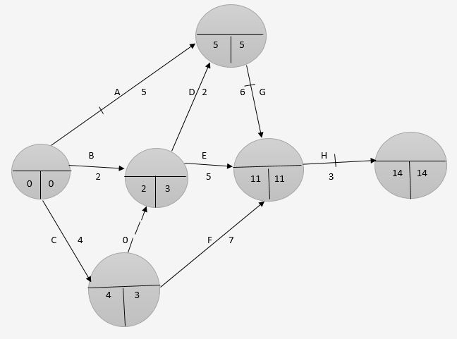
| Activity A B C D E F G H |
Duration (weeks) 5 2 4 2 5 7 6 3 |
Preceding activity - - - B B,C C A,D G, D, E, F |


| ➦ | Economics-September-2015-Pilot-Paper |
| ➦ | Economics-November-2015-Past-Paper |
| ➦ | Economics-May-2016-Past-paper |
| ➦ | Economics-November-2016-Past-Paper |
| ➦ | Economics-November-2017-Past-paper |
| ➦ | Economics-May-2017-Past-paper |
| ➦ | Economics-November-2018-Past-paper |
| ➦ | Economics-May-2018-Past-paper |
| ➦ | Economics-May-2019-Past-paper |
| ➦ | Economics-November-2019-Past-paper |
| ➦ | Economics-November-2020-Past-paper |
| ➦ | Economics-December-2021-Past-paper |
| ➦ | Economics-April-2021-Past-paper |
| ➦ | Economics-August-2021-Past-paper |

| ➧ | Introduction to Law and Governance-September-2015-Pilot-Paper |
| ➧ | Introduction to Law and Governance-November-2015-Past-Paper |
| ➧ | Introduction to Law and Governance-May-2016-Past-paper |
| ➧ | Introduction to Law and Governance-November-2016-Past-Paper |
| ➧ | Introduction to Law and Governance-May-2017-Past-paper |
| ➧ | Introduction to Law and Governance-November-2017-Past-Paper |
| ➧ | Introduction to Law and Governance-November-2018-Past-paper |
| ➧ | Introduction to Law and Governance-May-2018-Past-paper |
| ➧ | Introduction to Law and Governance-May-2019-Past-paper |
| ➧ | Introduction to Law and Governance-November-2019-Past-paper |
| ➧ | Introduction to Law and Governance-November-2020-Past-paper |
| ➧ | Introduction to Law and Governance-December-2021-Past-paper |
| ➧ | Introduction to Law and Governance-April-2021-Past-paper |
| ➧ | Introduction to Law and Governance-August-2021-Past-paper |
| ➧ | Financial Accounting -September-2015-Pilot-Paper |
| ➧ | Financial Accounting -November-2015-Past-Paper |
| ➧ | Financial Accounting -May-2016-Past-paper |
| ➧ | Financial Accounting-November-2016-Past-Paper |
| ➧ | Financial Accounting-November-2017-Past-paper |
| ➧ | Financial Accounting-May-2017-Past-paper |
| ➧ | Financial Accounting-November-2018-Past-paper |
| ➧ | Financial Accounting-May-2018-Past-paper |
| ➧ | Financial Accounting-May-2019-Past-paper |
| ➧ | Financial Accounting-November-2019-Past-paper |
| ➧ | Financial Accounting-November-2020-Past-paper |
| ➧ | Financial Accounting-December-2021-Past-paper |
| ➧ | Financial Accounting-April-2021-Past-paper |
| ➧ | Financial Accounting-August-2021-Past-paper |
CPA past papers with answers